Excel is the perfect tool for creating a Football Squares game board where you can easily update the numbers and participant numbers each game. It’s also great for sharing with your office pool. While it’s easy to simply create a 10×10 grid, I’m going to show you step by step how to build and format to make a spreadsheet you’ll be proud to share.
Here’s the quick steps on how to create your Excel football pool:
- Create a new blank worksheet in Excel.
- Type in the titles and numbers. Type the main title into E2, the Home Team into E4, and the Away Team into B6. Enter numbers 1 to 0 horizontally from E6 to N6. Then, do the same vertically from D7 to D16.
- Update font and adjust text sizes so that the title is the largest, team names next largest and then numbers.
- Update the column and row widths So that you have enough room to enter names into the numbered grids.
- Merge the cells for the headings so that titles are centered to the numbered grid. Merge the title and Home Team from column E to N. Merge the Away Team from row 7 to 16.
- Change the text orientation for the Away Team so that it’s 90 degrees or vertical. Vertically center as well.
- Add grid borders to the number grid to put a border around your 10×10 grid.
- Center grid cells both horizontally and vertically
- Optionally, add a light background to the numbers.
- Update the name cells to wrap text so that first and last names will fit within the table cell. Update the font size as needed.
There’s the basic instructions and you’ll find the full instructions below. I like to use Excel’s built-in formatting and structure as much as possible to save time but still end up with a great football grid that you can use again and again. Note: the instructions here are for Excel but the process would be similar for Google Docs, OpenOffice, or other spreadsheet solutions.
Full Instructions For Creating Football Squares in Excel
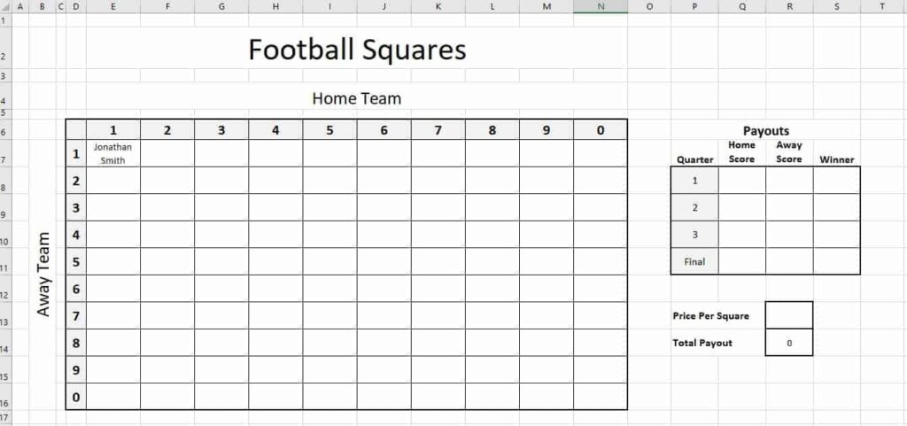
So before we get into the steps, here’s a screenshot of what we’re building. You can find a link to download it at the bottom.
First, create a new blank worksheet in Excel.
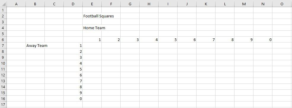
Then, type in the titles and numbers.
For now we’re just adding the titles and leaving room between for spacing. We’re adding the numbers 1 through 0 now in order but later, you can change them.
Update font and adjust text sizes.
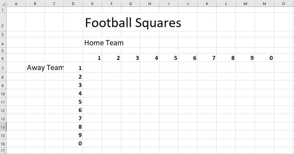
Before you go to much further, change your font if you’re going to. Each font will have its own size and spacing so it’s better to pick your font before you adjust your text sizes. For me, I’m keeping with the default Calibri since it’s super readable and looks fine.
Now you can update text sizes. In general, you’ll want to make the title the largest, the team names next largest and then the numbers. In my example below, I went with size 36 for the main title, size 24 for my team names, and 16 for the numbers. I also bolded the numbers.
Update the column and row widths.

This is where we start formatting the worksheet to look more like Football Squares. Adjust the widths of each column by hovering over the column borders in the gray header area and dragging. With Excel, it will actually tell you how many pixels if you want to get exact (which I do).
To quickly resize the number columns, you can select those columns and update the widths all at the same time.
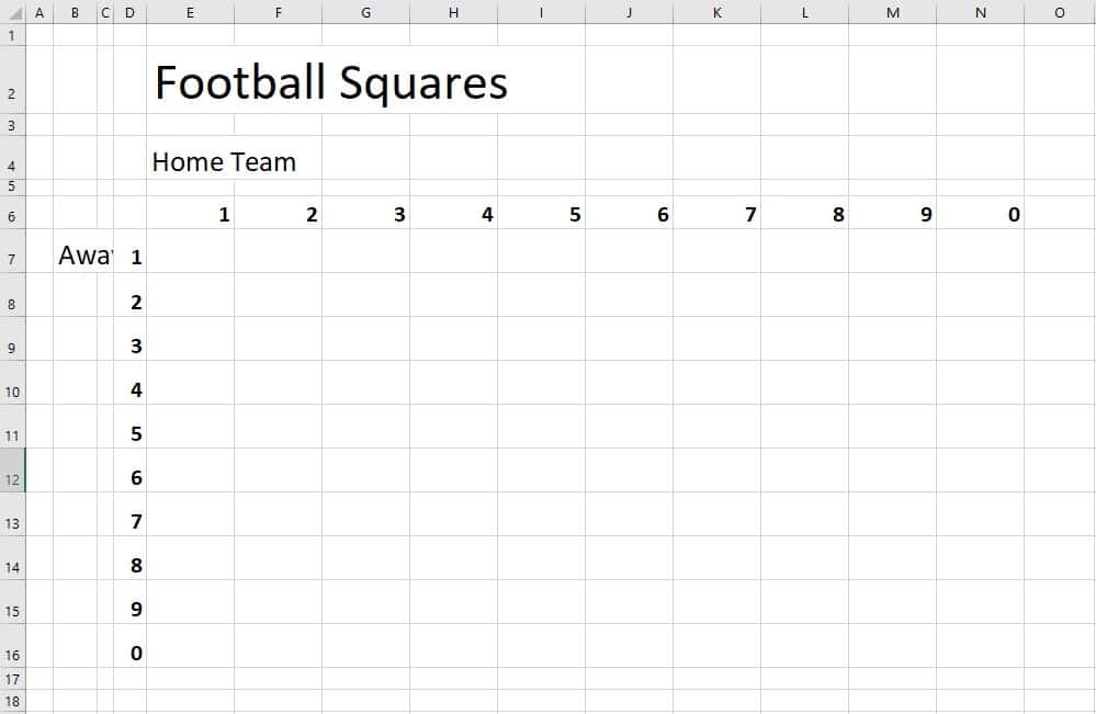
After you resize the columns, resize the rows in a similar manner. I usually set the row heights to be half the column widths for the numbers. That gives enough room to enter the names later.
Merge the cells for the headings.

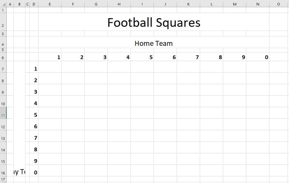
For both the main title and the team names, merge the cells for their areas. To do this, highlight the respective cells and then click on the Merge & Center button at the top.
After you do all three headings, it will look like this:
Change the text orientation for the Away Team.
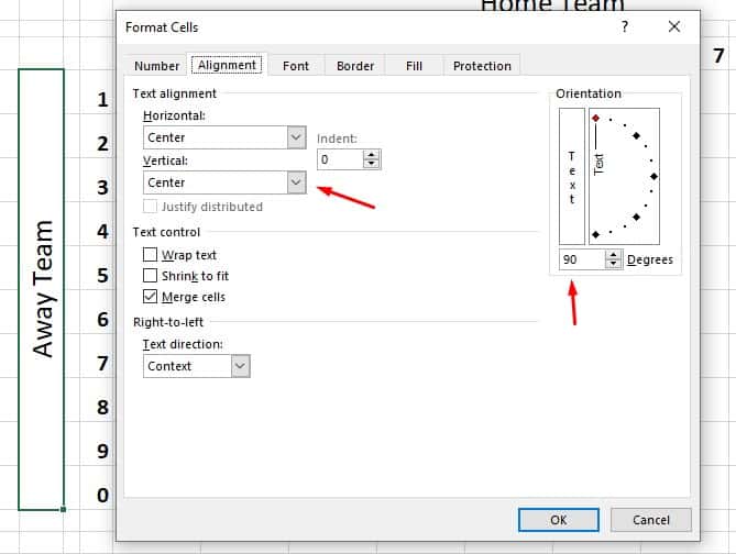
For the team name on the left, we need to update the text to read sideways. Right-click on the cell and select Format Cells. Go to the Alignment tab. Here, change the vertical alignment from Bottom to “Center”. Next, change the orientation from 0 degrees to 90 degrees.
Add grid borders.
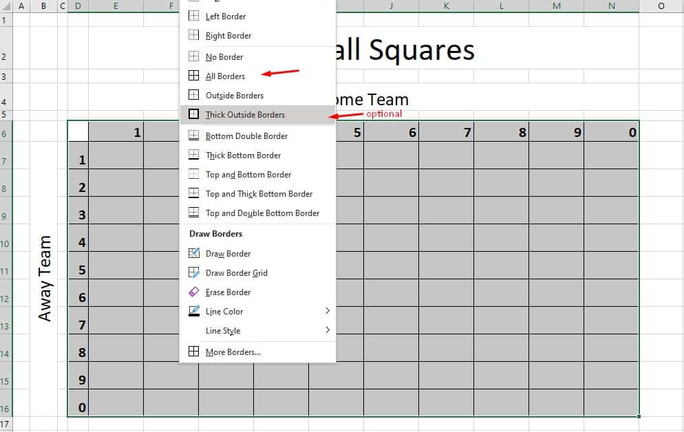
Select all the table cells that correspond to the numbers and where the names will go. This should be a big rectangle. Click on the borders icon in the toolbar and select borders for every side (All Borders). I like to also choose the thick border to go around the outside of the entire football grid.
Center grid cells.
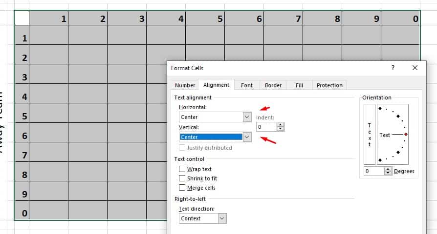
This will look better for the numbers and for the names that get entered into the “squares”. Select your grid, right-click and select Format Cells again. Set the horizontal and vertical alignment to be “Center”.
Add a light background to the numbers.
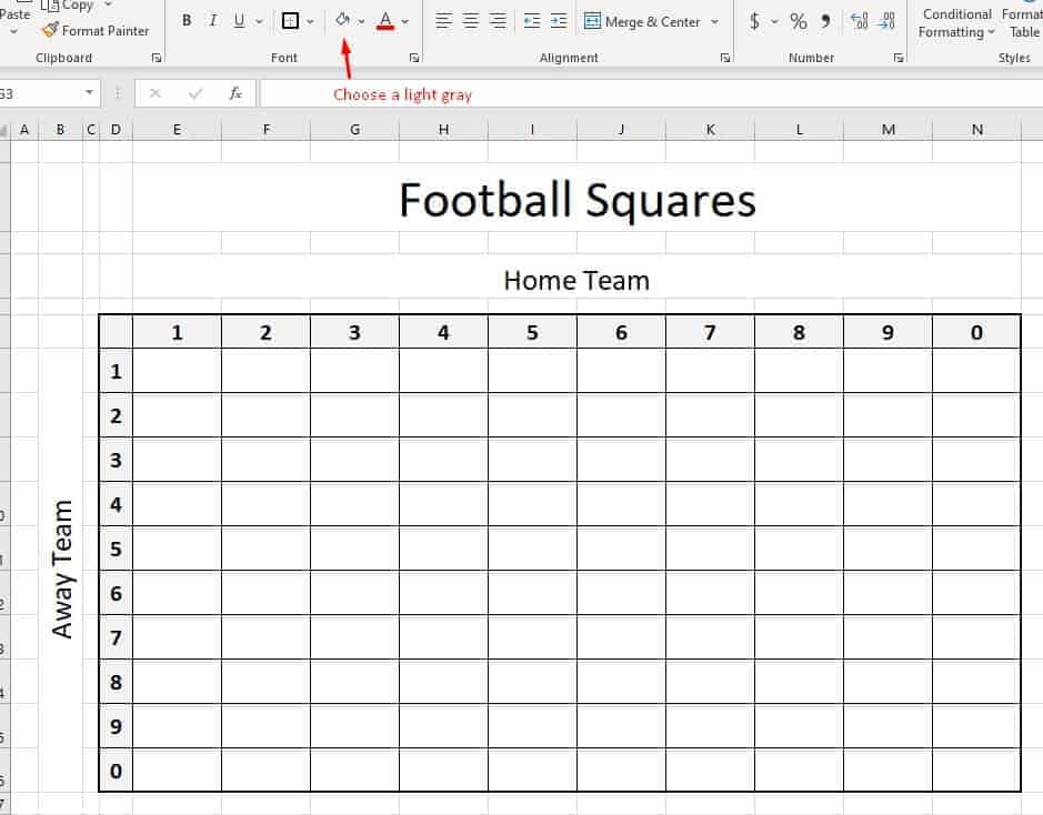
You don’t have to do this but it looks better. Simply select those cells and change the background color to a light gray.
Update the name cells to wrap text.
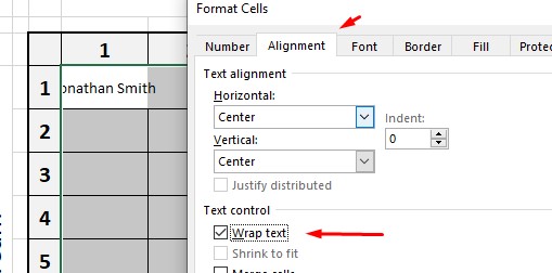
Enter a name into one of the squares so you can see how it’ll look. Then, select all the name boxes, right-click and click on Format Cells. Go to the alignment tab and click on the checkbox for Wrap text. Update the font size as needed.
That’s it, you just made a basic Football Squares pool that looks great. Before selling any squares, make sure to clear out the numbers. You can then print off your Excel sheet, or email it around to have each participant enter their name into the squares they want. After all squares have been filled, that’s when you’ll want to add the numbers 0 through 9 for both teams in random order. You can use my Football Squares random number generator to shuffle the numbers for you quick and easy.
Before I give you the link to download this spreadsheet, there’s a few more things I like to add. We have some space on the side so let’s add the price, pot, and payouts. I’m not going to give step by step instructions on these but they’ll be included in the final download. I prefer to do 4-quarter payouts so if you have a different payout, you can change that. The Total Payout will automatically calculate when you enter the Price Per Square.
If you’ve followed my step by step instructions and have created your own Excel football pool (or Football Squares), congratulations! If you’re not quite there, no worries – just download the finished spreadsheet below.
Download Football Squares Spreadsheet
Also check out the page Spreadsheet Templates for Football Squares for more advanced Excel and Google Doc options. For Google Docs, you can make a copy of my Google Sheets template for Football Squares.


